evomod2 simulates populations of diploid individuals whose multivariate phenotypes evolve under drift and Gaussian selection. Every simulation has the same three ingredients:
- a model: genetic architecture, mutation, recombination and environmental noise;
- a list of selection regimes;
- a call to
evolve(), which returns a population with statistics recorded along the way.
This vignette walks through each one with small, fast simulations.
The other vignettes compare genetic architectures
(vignette("architectures")) and reproduce the simulations
of Melo & Marroig (2015)
(vignette("melo-marroig-2015")).
Models
A genetic architecture says how genomes map to genotypic values \(x\). In the additive architecture, each allele carries an effect vector with one value per trait, and \(x\) is the sum of the effect vectors of all alleles. Mutation adds a multivariate normal vector to an allele’s effects.
model <- evomod_model(
  architecture = additive(loci = 20, traits = 4),
  mutation = mutation(rate = 0.005, cov = 0.1),  # cov: sd 0.1 per trait, uncorrelated
  env_sd = 0.8,                                  # phenotype z = x + Normal(0, 0.8^2)
  init_sd = 0.1                                  # starting allelic effects
)
model
#> <evomod model>
#>   architecture: additive - 20 loci, 4 traits
#>   mutation:     rate 0.005 per allele, random walk
#>   recombination: free
#>   life cycle:   wright_fisher
#>   env_sd:       0.8   init_sd: 0.1
Generations are discrete by default;
life_cycle = moran() gives overlapping generations, where
each generation is \(n\) birth-death
events (see ?life_cycles). Other architectures are
binary_b(), the binary ontogenetic matrix of the original
evomod model (with binary_b_mutation()), and
multilinear(), pairwise multilinear epistasis (see
?architectures). Loci recombine freely unless the model has
a genetic map (?recombination).
Selection regimes
Fitness is Gaussian around an optimum \(\theta\) (theta), with
covariance \(\Omega\)
(omega; larger \(\Omega\)
means weaker selection):
\[w(z) = \exp\left(-\tfrac{1}{2} (z - \theta)^\top \Omega^{-1} (z - \theta)\right)\]
omega <- diag(10, 4)
regimes <- list(
  drift(100),                                                  # no selection
  stabilizing(300, omega = omega),                             # fixed optimum
  directional(300, delta_theta = c(0.02, 0.02, 0, 0), omega = omega)  # moving optimum
)
directional() moves the optimum by
delta_theta every generation; here traits 1 and 2 are
pushed up while traits 3 and 4 stay put. fluctuating()
makes the optimum jump up or down every few generations, for all traits
together, independently, or in blocks (as in do O & Whitlock
2023):
fluctuating(5000, every = 10, step = 0.2, omega = 1, structure = list(1:2, 3:4))
#> <evomod regime> fluctuating for 5000 generations
Running a simulation
pop <- evolve(model, regimes, n = 300, record_every = 10, seed = 1)
pop
#> <evomod population> 300 individuals at generation 700
#>   architecture: additive - 20 loci, 4 traits
#>   regimes: drift (100), stabilizing (300), directional (300)
#>   records: 71 generations
Statistics are recorded every record_every
generations:
head(trait_means(pop))
#>   generation  trait       mean_x        mean_z theta
#> 1          0 trait1 -0.042971769 -0.0563562556     0
#> 2          0 trait2 -0.022712704 -0.0391483171     0
#> 3          0 trait3  0.008942121 -0.0153788330     0
#> 4          0 trait4  0.024249932  0.0858234510     0
#> 5         10 trait1  0.004493161  0.0004336258     0
#> 6         10 trait2 -0.061181608 -0.0014832862     0
tail(variances(pop))
#>     generation  trait         G         P        h2
#> 279        690 trait3 0.3717994 0.9405393 0.3953045
#> 280        690 trait4 0.4871923 1.0276138 0.4741006
#> 281        700 trait1 0.4140055 1.0076001 0.4108828
#> 282        700 trait2 0.4869124 1.2187075 0.3995318
#> 283        700 trait3 0.3761608 0.9690206 0.3881866
#> 284        700 trait4 0.5476366 1.2227502 0.4478728
g_matrices(pop)[["700"]]
#>              trait1       trait2      trait3      trait4
#> trait1  0.414005526 -0.007438328  0.02785657 0.103344112
#> trait2 -0.007438328  0.486912444 -0.10005839 0.008561561
#> trait3  0.027856569 -0.100058389  0.37616079 0.023234865
#> trait4  0.103344112  0.008561561  0.02323486 0.547636554
plot() shows mean genotypic values against the optimum,
additive variances, or a genetic correlation (grey lines mark the regime
boundaries):
plot(pop)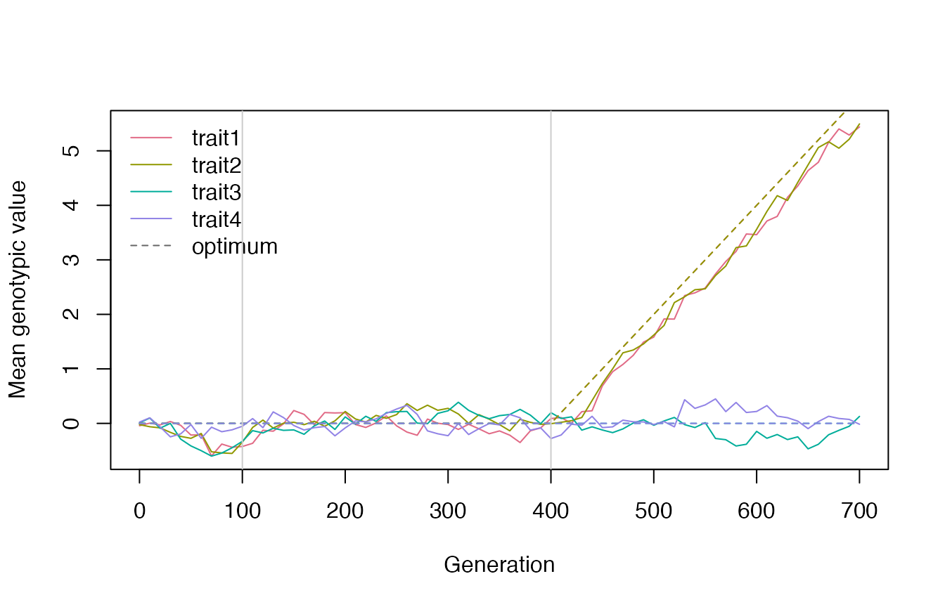
plot(pop, "variances")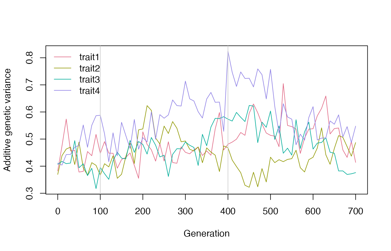
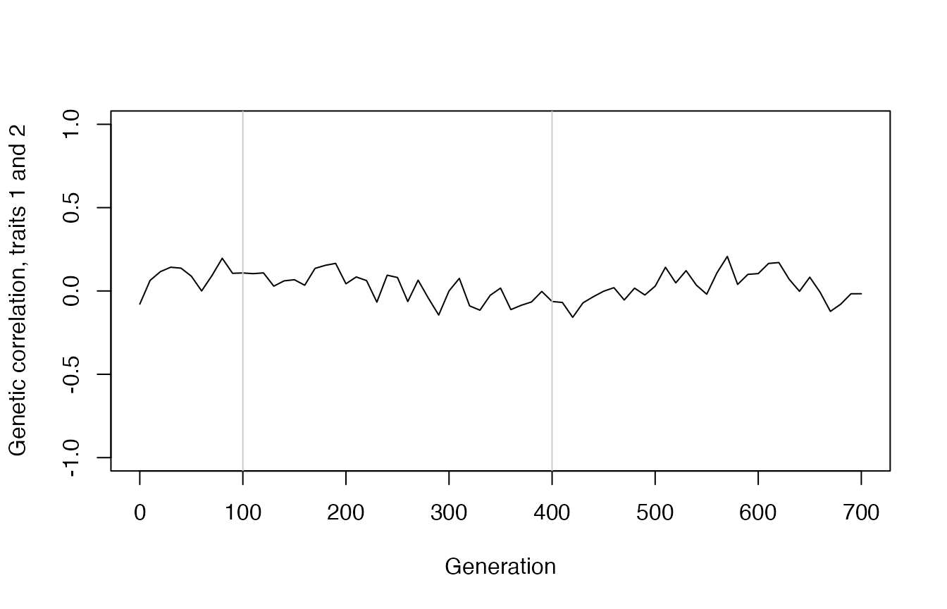
Continuing a population
evolve() also takes a population and continues it: same
individuals, generation count, optimum and records.
pop <- evolve(pop, stabilizing(200, omega = omega))
pop
#> <evomod population> 300 individuals at generation 900
#>   architecture: additive - 20 loci, 4 traits
#>   regimes: drift (100), stabilizing (300), directional (300), stabilizing (200)
#>   records: 91 generations
Runs are reproducible: random numbers come from R’s generator, so the
same seed (or set.seed()) gives the same
result, and continuing a population in two steps gives the same result
as running it in one.
Genomes and G matrix statistics
The current genomes are available as an array (rows x alleles x individuals; alleles \(2l - 1\) and \(2l\) are the two copies of locus \(l\)):
For architectures where genotypic values are sums of allele effects, G splits into a genic part (expected without linkage disequilibrium) and a linkage disequilibrium part:
dec <- g_decomposition(pop)
round(dec$genic, 3)
#>        trait1 trait2 trait3 trait4
#> trait1  0.409  0.012  0.022  0.102
#> trait2  0.012  0.400 -0.113 -0.013
#> trait3  0.022 -0.113  0.442  0.012
#> trait4  0.102 -0.013  0.012  0.640
round(dec$ld, 3)
#>        trait1 trait2 trait3 trait4
#> trait1 -0.029 -0.022  0.018  0.035
#> trait2 -0.022 -0.001  0.015 -0.073
#> trait3  0.018  0.015 -0.067  0.028
#> trait4  0.035 -0.073  0.028 -0.008
Matrix statistics for modularity and evolvability:
G <- dec$G
avg_corr(G, modules = list(1:2, 3:4))   # within- and between-module correlations
#> $within
#> [1] -0.02605202  0.08265489
#>
#> $between
#> [1] -0.009818828
#>
#> $avg_ratio
#> [1] -2.882364
autonomy(G, c(1, 1, 0, 0))               # autonomy in the direction of module 1
#> [1] 0.980875
mean_autonomy(G)                         # mean over random directions
#> [1] 0.9137727
eigen_variance(G)                        # proportion of variance per eigenvector
#> [1] 0.4095508 0.2504928 0.1902026 0.1497538
Larger simulations
The examples in
system.file("examples", package = "evomod2") run larger,
replicated experiments from the command line, one replicate per process,
so they can run in parallel:
list.files(system.file("examples", package = "evomod2"))
#> [1] "corridor_linkage.R"         "corridor_selection.R"
#> [3] "fluctuating_environments.R" "jones_burger_arnold_2014.R"
#> [5] "melo_marroig_2015.R"